
In this project, I have built a real-life data science project called "real estate house price prediction. " This model can predict the property prices based on certain features such as square feet, bed room, bathroom, location, etc
To make this project fun, I have built a website using HTML, CSS, and JavaScript that can provide home price predictions for us in the form of project architecture.
Frist I have downloaded a data set from Kaggle.com. This data set is about Bengaluru, India.
By using this data set, I have built a machine learning model. This model has covers some of the cool data science concepts such as DATA CLEANING, DIMENSIONAITY OF REDUCTION, OUTLIERS REMOVAL, ONEHOT ENCODING, GRIDSEARCHCV
I have written a Python Flask server that can consume this pickle file and do price prediction. This Python Flask server will expose http end points for various requests, and the user interface written in HTML, CSS, and JavaScript will make HTTP GET and Post Calls in terms of tools.
For this project, I have used Python as a programming language, Pandas for data cleaning, Matplotlib for data visualization, Sklearn for model building, and Python Flask for the backend server.
* Project Begining *
Step:-1 Data Cleaning
I have downloaded the data set into Pandas to perform data cleaning using cool techniques.
My data set looks like this: I have the area type of the liberty location size, the square foot area, etc., and all these are independent variables, and my dependent variable is price. "Price is something that I have to predict."
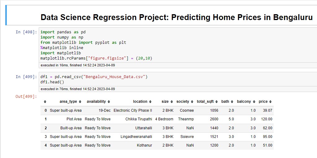
I am using supervised learning here (linear regression), and all label data basically has input and output values based on that. I have created a new Jupyter notebook for model building and imported a few basic libraries like Pandas, Numpy, and Matplotlib, as shown in the above picture.
After importing these libraries, I have the csv file loaded into the Pandas data frame. "You can see the data frame loaded without the data from the csv file." To see the number of rows and columns in the data set, we can use the shape command. Here, I have 13 thousand rows, which is a decent enough data set.
Frist I have examined the Area Type feature to keep my model simple. I had dropped certain columns from the data, like "area type, city, balcony, availability." After that, my data frame looked like this after using this funtion
df2 = df1.drop([
                  'area_type','society','balcony','availability'
                  ],axis='columns'
                  )
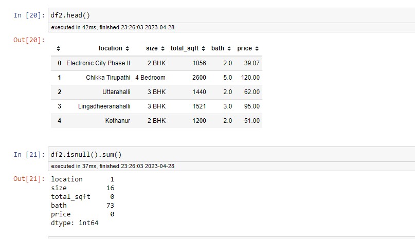
The data cleaning process starts with handling missing values by using isnull(). I have found that in 73 rows where the value of the bath room is not available, as I have 13 thousand rows, it is safe to drop. After dropping the null values, I have created a new data frame.
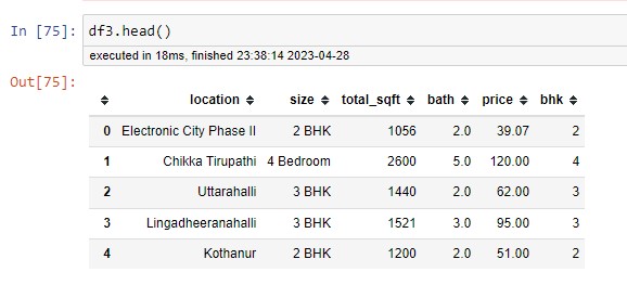
I have explored the "SIZE" feature by applying a unique function. I noticed that 4 bhk and 4 bed rooms are the same but considered two different features. To eliminate this problem, I have created a new column, "BHK." This column is based on the "size" column
df3['bhk'] = df3['size'].apply(lambda x: int(x.split(' ')[0]))
This function accepts the string, tokenizes it using space, and takes the first token and converts it into an integer.
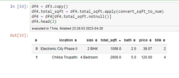
Similarly, when exploring the "total_sqft" column, I have found that there are some range values. I want to convert the range values to a single number by taking the average of the two numbers.
                      def is_float(x):
                      try:
                          float(x)
                      except:
                          return False
                      return True
Below function will take the range as an input and return the average value. If you take an input string, split it using (-). Now we have two individual numbers that are taken into float numbers, and then we take the average; otherwise, it will convert the normal number into a float number. I applied this function to a square-foot column and created a new data frame. DF4 is a deep copy of DF3.
                      def convert_sqft_to_num(x):
                      tokens = x.split('-')
                      if len(tokens) == 2:
                          return (float(tokens[0])+float(tokens[1]))/2
                      try:
                          return float(x)
                      except:
                          return None
Step:-2 Feature Engineering
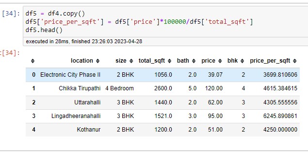
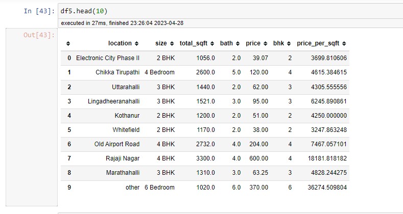
Now that I have created a new column "Price per Square Foot", we all know that in the real estate market, the price per square foot is very important. This feature will help us find the outliers in the later stages. The new column is noting the division of the two columns "Price" and "Square foot area."
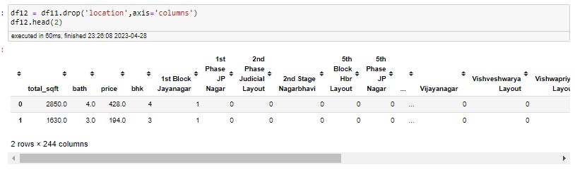
Now, when exploring the location column, first check how many locations I have in total because if we have too many locations, it will create a problem. By applying the unique function to the location, I have found thirteen thousand locations. To handle the text data, we use ONEHOTENCODING to convert them into dummy columns. If we keep all the locations, we will have around 1300 columns, which is just too much, like too many features. This is called the "dimensionality curse."
There are some techniques available to reduce the dimension. One of the best techniques to come up with this "Other Category" is that we had 1304 locations and found that there are many locations with one or more data points.
                    df5.location = df5.location.apply(lambda x: 'other' if x in location_stats_less_than_10 else x)
                      len(df5.location.unique())
Step:-3 Outliers Detection
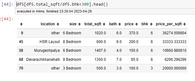
In this stage, the outlier detection and removal outliers are the data points that are the data errors, or sometimes they are not data errors but they just represent the extreme variation; it makes sense to remove them otherwise they create some issues later on. We can apply simple domain knowledge or the standard deviation. The real estate domain is that when you have two bed rooms in an apartment, for example, for a single bed room, there is a threshold limit of 300 square feet per bed room; more than that is unusual. I had to remove all these unusual data points with this function.
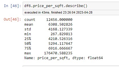
When I am checking the price per square foot I found some properties that were very high or very low. By describing a method on a particular column, we get statistics for that column. Where 267 Rs per square foot is very low and similarly the property price of 176470 is very high, it is possible If its a prime area, but we are building a generic model, I thought it made sense to remove this kind of extreme case. By creating a function based on the standard deviation
Below function will take the data frame as input, grouping them by location frist and poor location. This will create a sub-data frame for which I am calculating mean M and standard deviation and then filtering all these data points beyond the standard deviation, which means anything above mean minus one standard deviation and anything below mean plus one standard deviation, I will keep it in my reduced data frame and then keep appending those dataframe per location, and this will give me the output data frame, which I will call DF7 This function will remove 2000 outliers from our data set.
                      def remove_pps_outliers(df):
                      df_out = pd.DataFrame()
                      for key, subdf in df.groupby('location'):
                          m = np.mean(subdf.price_per_sqft)
                          st = np.std(subdf.price_per_sqft)
                          reduced_df = subdf[(subdf.price_per_sqft>(m-st)) & (subdf.price_per_sqft<=(m+st))]
                          df_out = pd.concat([df_out,reduced_df],ignore_index=True)
                      return df_out

                     df7 = remove_pps_outliers(df6)
                     df7.shape
One more thing in our data set: the property prices for a 3-bedroom apartment are higher than the property prices of a 2-bedroom apartment for the same square foot area
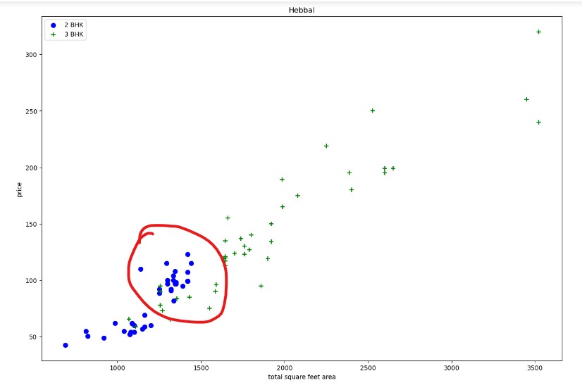
For example, here we are looking at two properties with the same square feet, around 1200 square feet, but I saw that the 3 bed room price is 81 lakhs, whereas the 2 bed room price is 27 lakhs, so although the square field is the same, with a smaller number of bed rooms, the property price is high. This could be due to many reasons; it could be some locations where there are some special amenities, or anything else. To find out how many such cases are available in the data set, I wrote a function that will scatter plot to give me a visualisation. The function will draw a scatter plot on which it will plot two-bedroom apartments and three-bedroom apartments. This function will take a data frame and location as input.
                      def remove_bhk_outliers(df):
                      exclude_indices = np.array([])
                      for location, location_df in df.groupby('location'):
                          bhk_stats = {}
                          for bhk, bhk_df in location_df.groupby('bhk'):
                              bhk_stats[bhk] = {
                                  'mean': np.mean(bhk_df.price_per_sqft),
                                  'std': np.std(bhk_df.price_per_sqft),
                                  'count': bhk_df.shape[0]
                              }
                          for bhk, bhk_df in location_df.groupby('bhk'):
                              stats = bhk_stats.get(bhk-1)
                              if stats and stats['count']>5:
                                  exclude_indices = np.append(exclude_indices, bhk_df[bhk_df.price_per_sqft<(stats['mean'])].index.values)
                      return df.drop(exclude_indices,axis='index')
                      df8 = remove_bhk_outliers(df7)
                       #df8 = df7.copy()
                      df8.shape
Here, the blue points are two-bedroom apartments and the green markers are three-bedroom apartments, where the X-axis has the total square foot area and the Y-axis has the price per square foot. If we look at the vertical line for the same square foot area, this particular line (1700 square foot area) shows that the two-bedroom price is higher than the three-bedroom price. I have these four data points that are considered outliers. For these outliers, I have written a function that creates two different sets of data for the same location, which will have data points for a two-bedroom and a three-bedroom apartment. again plotting the same scatter plot to see what kind of improvement it has made.
                      def plot_scatter_chart(df, location):
                      bhk2 = df[(df.location==location) & (df.bhk==2)]
                      bhk3 = df[(df.location==location) & (df.bhk==3)]
                      matplotlib.rcParams['figure.figsize']= (15,10)
                      plt.scatter(bhk2.total_sqft,bhk2.price,color='blue',label='2 BHK', s=50)
                      plt.scatter(bhk3.total_sqft,bhk3.price,marker='+',color='green',label='3 BHK', s=50)
                      plt.xlabel('total square feet area')
                      plt.ylabel('price')
                      plt.title(location)
                      plt.legend()
                      plot_scatter_chart(df7, "Hebbal")
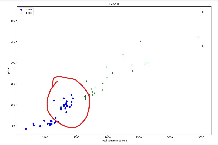
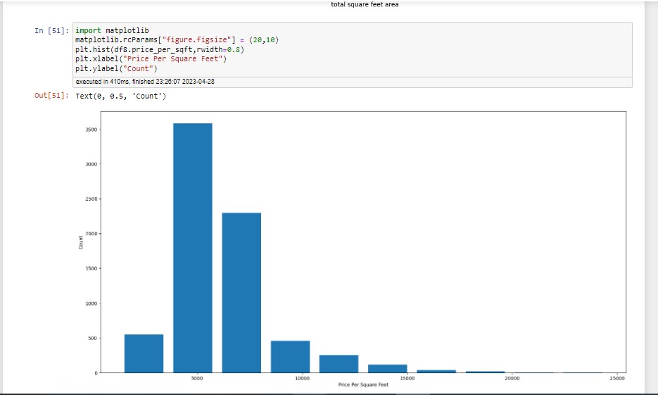
We can see these green data points in the previous plot; those data points are gone now, and the majority of three-bedroom apartments have a higher value. After removing the outliers, I want to see how many apartments or properties I have per square foot.
We can see the x-axis has the majority of the property and the y-axis has the price per square foot. It shows the number of data points in the category, like 0 to 10000 per square foot. In the majority of my data points, we can see a normal distribution, kind of like a Guassian cure.
Now we are going to explore bathroom features. When I applied the unique value function, I found that there are 12 bathrooms and more. According to the real estate domain knowledge, the number of bathrooms is greater than bed rooms plus two. We are going to remove those as outliers. This function will remove those outliers.
df9 = df8[df8.bath'<'/df8.bhk+2]
I still have around seven thousand data points in that now my data frame looks pretty much neat and clean, so I know I can start preparing it for machine learning training, and for that I have to drop some unneeded features, so the price per square foot and size feature are unneeded at this point because size is already a BHK feature, so this one can be dropped because it is used for outliers.
Leave a Reply